What Is Adaline?
ADAptive LInear NEuron (Adaline)
Adaline can be thought of as an improvement on the perceptron. If you don’t know what a perceptron is, then I would highly suggest you read my blog article on it here. Adaline was published a couple of years after the perceptron algorithm by Rosenblatt. It was published by Bernard Widrow and his doctoral student Tedd Hoff. It was published in October of 1960.
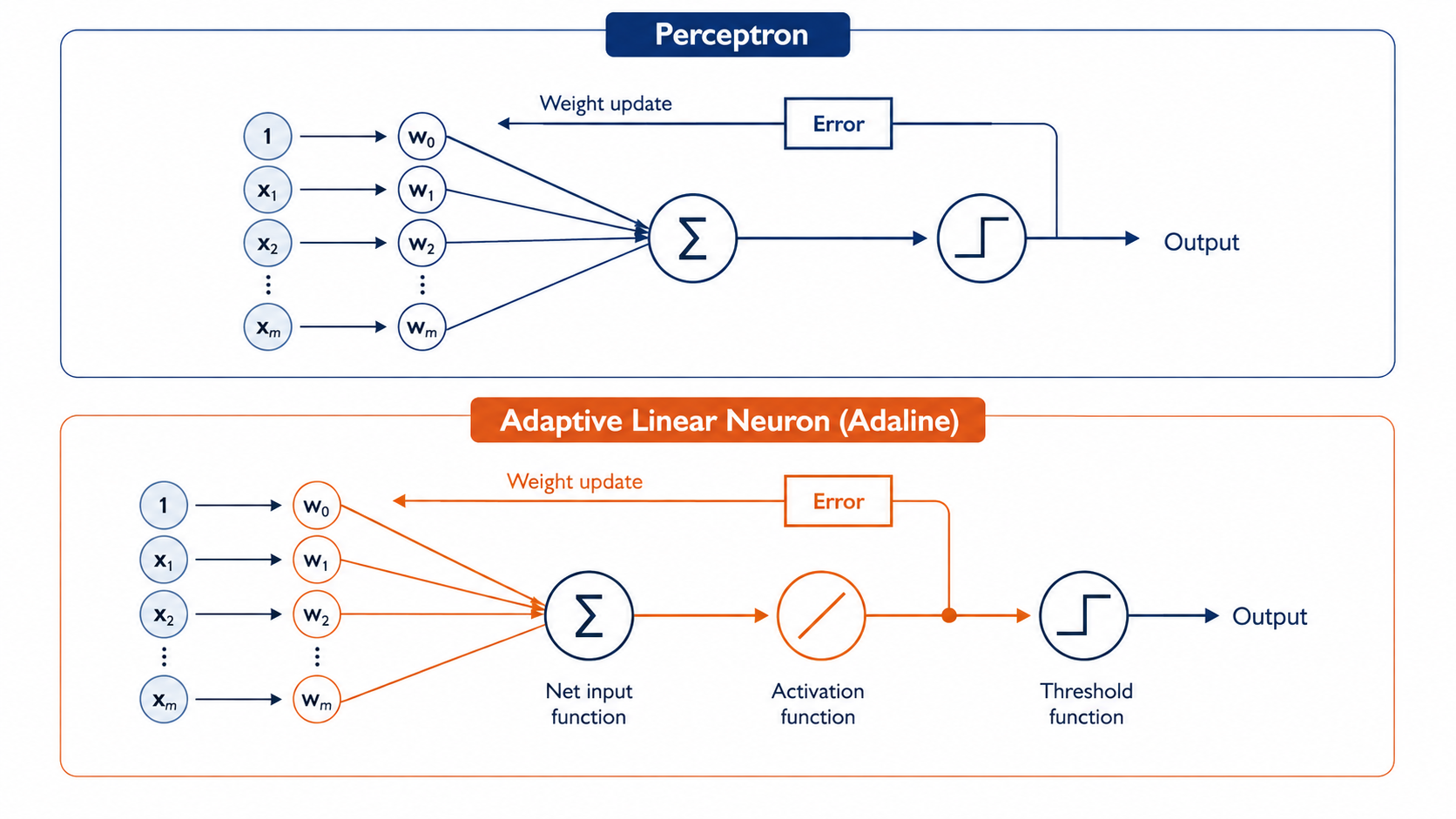
There are some key differences between Adaline and the perceptron. The first one that I will mention is that Adaline introduces the concept of defining and minimizing a continuous cost function. The second difference in Adaline is that the weights are updated based on a linear activation function as opposed to the unit step function that is used in the perceptron. In Adaline the linear activation function is simply the net input as shown below.
\[ \phi(\textbf{w}^T \textbf{x}) = \textbf{w}^T \textbf{x} \]
Here, \(\textbf{w}^T\) is the vector of model weights and \(\textbf{x}\) is a training example.
In Adaline there is the linear activation function, which is shown above. Then there is the threshold prediction function which the unit step function and is used to make predictions after the model has been trained. We can see the differences in the illustration shown below.
Minimizing The Cost Function With Gradient Descent
In supervised machine learning there is a defined objective function that we optimize for during the learning proccess. In this case for Adaline, the objective function is the cost function below.
\[J(\textbf{w}) = \frac{1}{2}\sum_i (y^{(i)} - \phi{(z^{(i)})})^2\]
I want to quickly note before moving forward that \(z^{(i)} = \textbf{w}^T \textbf{x}^{(i)}\). Here \(\textbf{w}^T\) is the vector of weights and \(\textbf{x}^{(i)}\) is the vector of the \(i^{th}\) training example.
The function \(J\) is simply the sum of squred errors between the output of the activation function and the true class label. The \(\frac{1}{2}\) term in the function is added for convenience and will make calculating the gradient much easier with respect to the weights. The main advantage of the continuous linear activation, compared to the unit step function, is that it makes the cost function differentiable. Another property of the cost function is that it is convex. This allows us to use the gradient descent algorithm to find the weights that minimize the cost function.
So what is gradient descent? Gradient descent is an optimization algorithm that helps us minimize a cost function. As the name implies, it uses the gradient to accomplish this. A question you might ask then is what is a gradient. The gradient is a vector of partial derivatives of a function. For example, with the cost function \(J\) we would have the following.
\[ \nabla J(\mathbf{w}) = \begin{bmatrix} \frac{\partial J}{\partial w_1} \\[6pt] \frac{\partial J}{\partial w_2} \\[6pt] \vdots \\[6pt] \frac{\partial J}{\partial w_m} \end{bmatrix} \]
Each element in the vector is the partial derivative of the cost function with respect to a particular weight.
So what information does the gradient give us? The gradient points in the direction of steepest ascent. Thereofore, by moving in the opposite direction we will end up moving towards a point that should minimize the cost function even further.
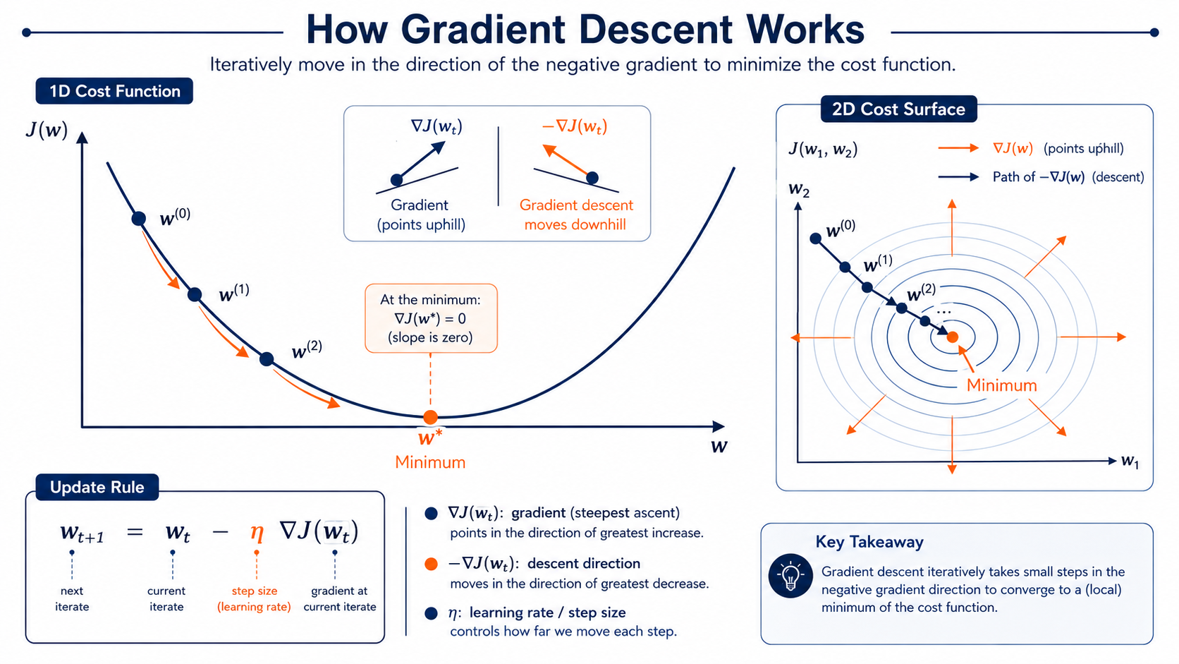
Our cost function is \(J(\textbf{w})\) and the update rule would be the following.
\[\textbf{w} := \textbf{w} + \Delta \textbf{w}\]
\(\delta \textbf{w}\) is the change in weights and is defined as the negative gradient multiplied by the learning rate.
\[\Delta \textbf{w} = -\eta \nabla J(\textbf{w})\]
In order to compute the gradient of the cost function, we need to compute the partial derivative of the cost function with respect to each weight, \(\textbf{w}_j\):
\[\frac{\partial J}{\partial w_j} = -\sum_i \left( y^{(i)} - \phi(z^{(i)}) \right)x_j^{(i)}\]
The update of \(w_j\) could then be written as:
\[\Delta w_j = -\eta \frac{\partial J}{\partial w_j} = \eta \sum_i \left( y^{(i)} - \phi(z^{(i)}) \right)x_j^{(i)}\]
On a quick note. The Adaline and perceptron learning rules look similar but are different. The Adaline learning rule uses \(\phi(z^{(i)})\) with \(z^{(i)} = \textbf{w}^T \textbf{x}\) which is a real number and not an integer class label. Adaline also updates the weights using all of the training examples in the dataset instead of updating the weights incrementally after each training example like in the perceptron algorithm.
Code Example
class AdalineGD(object):

    def __init__(self, eta = 0.01, n_iter = 50, random_state = 1):
        self.eta = eta
        self.n_iter = n_iter
        self.random_state = random_state

    def fit(self, X: np.ndarray, y: np.ndarray):

        rgen = np.random.RandomState(self.random_state)
        self.w_ = rgen.normal(loc=0.0, scale=0.01, size=1 + X.shape[1])

        self.cost_ = []

        for i in range(self.n_iter):
            net_input = self.net_input(X)
            output = self.activation(net_input)
            errors = (y - output)
            self.w_[1:] += self.eta * X.T.dot(errors)
            self.w_[0] += self.eta * errors.sum()
            cost = (errors**2).sum() / 2.0
            self.cost_.append(cost)

        return self

    def net_input(self, X: np.ndarray):
        return np.dot(X, self.w_[1:]) + self.w_[0]

    def activation(self, X: np.ndarray):
        return X

    def predict(self, X: np.ndarray):
        return np.where(
            self.activation(self.net_input(X)) >= 0.0,
            1,
            -1
        )
Above we have an implementation of Adaline in python. I will explain the code as best as I can. If I have made any errors in this blog post, please feel free to reach out to me and correct me. This code is from the book Python Machine Learning and can be found here
When the class is created we must pass in the learning rate \(\eta\), the number of iterations that the algorithm will loop through to update the weights, and the random state which will allow for reproducible results.
I will start by explaining the fit function since that is where everything is happening in this example.
In the beginning of the function we have the following three lines of code.
rgen = np.random.RandomState(self.random_state)
self.w_ = rgen.normal(loc=0.0, scale=0.01, size=1 + X.shape[1])

self.cost_ = []
The first line initializes the random number generator so that we can generate random weight values. The second line actually generates the random values from a normal distribution. Lastly, we create an empty list that will hold the values of the cost function for each iteration of the training step.
The fit function then enters a for loop that loops n_iter times. The function first calculates \(\phi(z^{(i)})\) where \(z^{(i)} = \textbf{w}^T
\textbf{x}^{(i)}\). This is done using the net_input function which calculates the dot product between the weights and every training example. Mathematically is does the following:
\[\textbf{w}^T \textbf{x}^{(i)}\]
for each \(i\) from the first example to the last. This is all done easily in a vectorized form using numpy’s dot function. In the code
net_input = self.net_input(X)the numpy array X is an \(n\) by \(m\) array where \(n\) is the number of training examples and \(m\) the number of features.
In the net_input function we have the single line of code:
return np.dot(X, self.w_[1:]) + self.w_[0]Here the dot product is calculated between every row in X and the weights from 1 to m. This is why you see self.w_[1:] because it excludes the bias weight which is added after the dot product. This is done because the weight vector is actualy of dimension \(m+1\) where as the matrix X is of dimensions \(n \times m\). This makes sense if we imagine adding an additional column with just 1’s as the entries as the first column of X.
Then we have the next line in the fit function:
output = self.activation(net_input)Here the activation function is just the identity function, which can clearly be seen by its only line of code. This is not strictly needed but it closely resembles the mathematics.
The next line of code, shown below, just calculates the errors which is the difference between the actual values and the values generated by the function \(\phi\).
errors = (y - output)Here y and output are actually vectors of length \(n\). So the difference is calculated for all the values simultaneously.
The following line will require much more explination as this is where we are updating all of the weights at the same time. I will do my best here to explain it.
self.w_[1:] += self.eta * X.T.dot(errors)The majority of the work is being done in the following part of the line of the code, X.T.dot(errors). Here we are taking the matrix X which is \(n \times m\) and transposing it. This turns the columns/features into rows. So if X.shape == (100,2) then X.T.shape == (2,100). Cenceptually, if:
X =
[
  [x11, x12],
  [x21, x22],
  [x31, x32]
]
then:
X.T =
[
  [x11, x21, x31],
  [x12, x22, x32]
]
Now each row of X.T contans all the values for one feature.
Then we take the dot product of the transposed matrix X with vector of errors. What is happening here is that dot product is being taken between the vecotr of errors and each row.
So suppose:
X.T.shape == (2, 100)
errors.shape == (100,)
then:
X.T.dot(errors).shape == (2,)The result is a vector with one value per feature.
It computes:
[
  x11*error1 + x21*error2 + ... + x100,1*error100,
  x12*error1 + x22*error2 + ... + x100,2*error100
]
Or more generally:
\[\Delta w_j = \eta \sum_i x_j^{(i)}\left(y^{(i)} - \hat{y}^{(i)}\right)\]
What’s being computed here is the summation.
Then it is multiplied by the learning rate, self.eta. Lastly, it all gets added to the current weights self.w_[1:].
The bias unit is handled separately with the following line:
self.w_[0] += self.eta * errors.sum()Lastly, the cost is computed for the current iteration and added to the cost array to keep track of how the cost is changing.
cost = (errors**2).sum() / 2.0
self.cost_.append(cost)
The last function to understand is the predict function. This function make a prediciton based on the value of the activation function. If the value is greater than or equal to 0 then a value of ` is returned and -1 otherwise. These are the class labels.
There you have it. I have tried my best to explain what Adaline is and how it works.